Usage
Installation
It is recommended you use voxelmap through a virtual environment. You may follow the below simple protocol to create the virtual environment, run it, and install the package there:
$ virtualenv venv
$ source venv/bin/activate
(.venv) $ pip install voxelmap
To exit the virtual environment, simply type deactivate. To access it at any other time again, enter with the above source command.
The hashblocks Constructor Variable
Voxelmap was originally made to handle third-order integer arrays of the form np.array((int,int,int)) as blueprints to 3-D voxel models.
While “0” integers are used to represent empty space, non-zero integers are used to define a distinct voxel type and thus,
they are used as keys for such voxel type to be mapped to a specific color and alpha transparency. These keys are stored in a map (also known as “dictionary”)
internal to the voxelmap.Model class called hashblocks.
The hashblocks dictionary contains an entry for each integer key,
where the corresponding value is a list. This list contains two elements:
a string that represents the color in either the hex format (#rrggbb) or as a color label (e.g., ‘red’)
as the first element, and a float between 0 and 1 that represents the alpha transparency as the second element.
The dictionary’s structure and call method are shown below:
import voxelmap as vxm

model = vxm.Model()

model.hashblocks = {
   key_1 (int): ['#rrggbb' (string) ,alpha (float)]
   key_2 (int): ['#rrggbb' (string) ,alpha (float)]
   .
   .
   .
}
Draw voxels from integer arrays
We present the creation of two models using arrays A and B, with the first code block dedicated to the generation of the first model (array A) containing thorough comments for better understanding of the voxelmap functions.
'''Array A'''

#make a 10x10x10 integer array with values between 0 and 3 with sampling probabilities "p"
freqs = [300,20,40,20]
A = np.random.choice([0,1,2,3],p=freqs/np.sum(freqs),size=(10, 10, 10))

#incorporate array to Model structure
model = vxm.Model(A)

#add voxel colors and alpha-transparency for integer values 0 - 9 (needed for `custom` coloring)
colors = ['#ff000ff', 'yellow', 'lime']

alpha_yellow=0.4    # define alpha transparency for yellow colored voxels

#assign colors and alpha to integers
k=1
for i in colors:
    model.hashblocks[k] = [i,1] if i != 'yellow' else [i,alpha_yellow]
    k+=1

model.draw(coloring='custom',len_voxel=0.9, background_color='#ffffff')

'''Array B'''

B = np.random.randint(1,30,(7,7,7))
vxm.Model(B).draw(coloring='cmap: cool, alpha:1.0',geometry='particles',len_voxel=1,background_color='w')
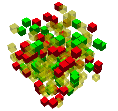
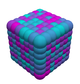
It’s worth noting the versatility of voxelmap, allowing the creation of 3D models using just one line of code, as demonstrated with the generation of array B.
Draw voxels from coordinate arrays
Voxelmap has the capability to create a voxel model using an array that defines the coordinates of each voxel in x, y, and z space. The variable “data.xyz” takes a third-order array, where the rows represent the number of voxels and the columns contain the 3 coordinates for each axis.
Additionally, the “data.rgb” input can be used to set the color of each voxel in the “data.xyz” object using the hex format “xxxxxx” (for example, “ffffff” for white).
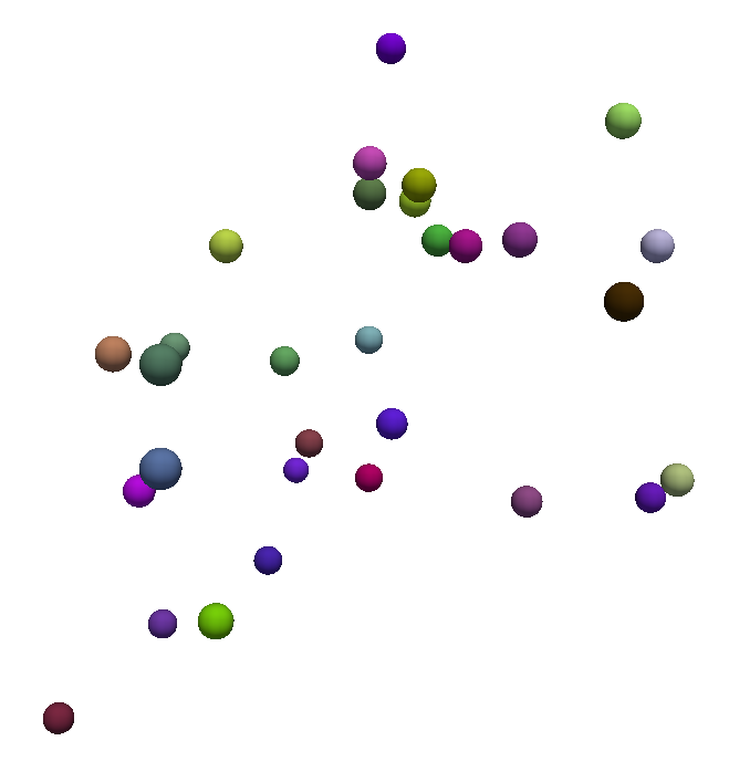
The algorithm works with negative coordinates as well, as demonstrated in the example below. This example showcases two cases, where the second case places the spheres farther apart by reducing the characteristic length scale of the particles (i.e., the radius) using the “len_voxel” keyword argument.
cubes = vxm.Model()
num_voxels = 30
cubes.XYZ = np.random.randint(-1,1,(num_voxels,3))+np.random.random((num_voxels,3))          # random x,y,z locs for 10 voxels
cubes.RGB = [ hex(np.random.randint(0.5e7,1.5e7))[2:] for i in range(num_voxels) ]   # define random colors for the 10 voxels
cubes.sparsity = 10
                                                  # spaces out coordinates
cubes.load(coords=True)
cubes.hashblocks

print(cubes.hashblocks)

# print(cubes.XYZ)                               # print the xyz coordinate data
cubes.draw(coloring='custom',geometry='particles',len_voxel=1, background_color='#ffffff',window_size=[416, 416])

# increase spacing by setting the `len_voxel` characteristic side-length to a lower number.
cubes.draw(coloring='custom',geometry='particles',len_voxel=0.5, background_color='#ffffff',window_size=[416, 416])
>>> [Out]
Voxelmap draw. Using custom colors:
self.hashblocks =
 {1: ['#4d3206', 1], 2: ['#4f29cc', 1], 3: ['#52c64a', 1], 4: ['#5c8c76', 1], 5: ['#617fc0', 1], 6: ['#6622fa', 1], 7: ['#668b58', 1], 8: ['#6cb872', 1], 9: ['#701eda', 1], 10: ['#76aa8b', 1], 11: ['#783ec3', 1], 12: ['#7b2af8', 1], 13: ['#80e30b', 1], 14: ['#8105f8', 1], 15: ['#842c4c', 1], 16: ['#89c2d5', 1], 17: ['#934959', 1], 18: ['#9a539c', 1], 19: ['#9f3fae', 1], 20: ['#a5b909', 1], 21: ['#a9f373', 1], 22: ['#b818a6', 1], 23: ['#bcf032', 1], 24: ['#bd0374', 1], 25: ['#bdd493', 1], 26: ['#c20eff', 1], 27: ['#c9c6fe', 1], 28: ['#c9ea55', 1], 29: ['#cc8e6f', 1], 30: ['#d553d4', 1]}
Colormap Block Coloring
The coloring kwarg for the draw method now has a 'cmap' string option to assign colors from a colormap to the defined voxel types (i.e. the
non-zero integers in the 3-D arrays). Download the RANDOMWALK.JSON file
and save it in the same directory where you are running these examples. If you inspect the .json file, you’ll see the following structure:
{
   "hashblocks": {},
   "size": [300, 300, 300],
   "coords": [
      [146, 149, 152],
      [146, 150, 152],
      [147, 148, 153],
      [147, 148, 154],
      .
      .
      .
      [197, 142, 132],
      [197, 143, 132]
   ],
   "val": [7, 6, 24, 25, . . ., 3182, 3183]
}
The file contains information about a 3-D array, including its dimensions (specified by the size key),
the 3-D coordinates of its non-zero integers (specified by the coords key), and the corresponding integer values (specified by the val key).
It’s worth noting that the hashblocks dictionary is currently empty.
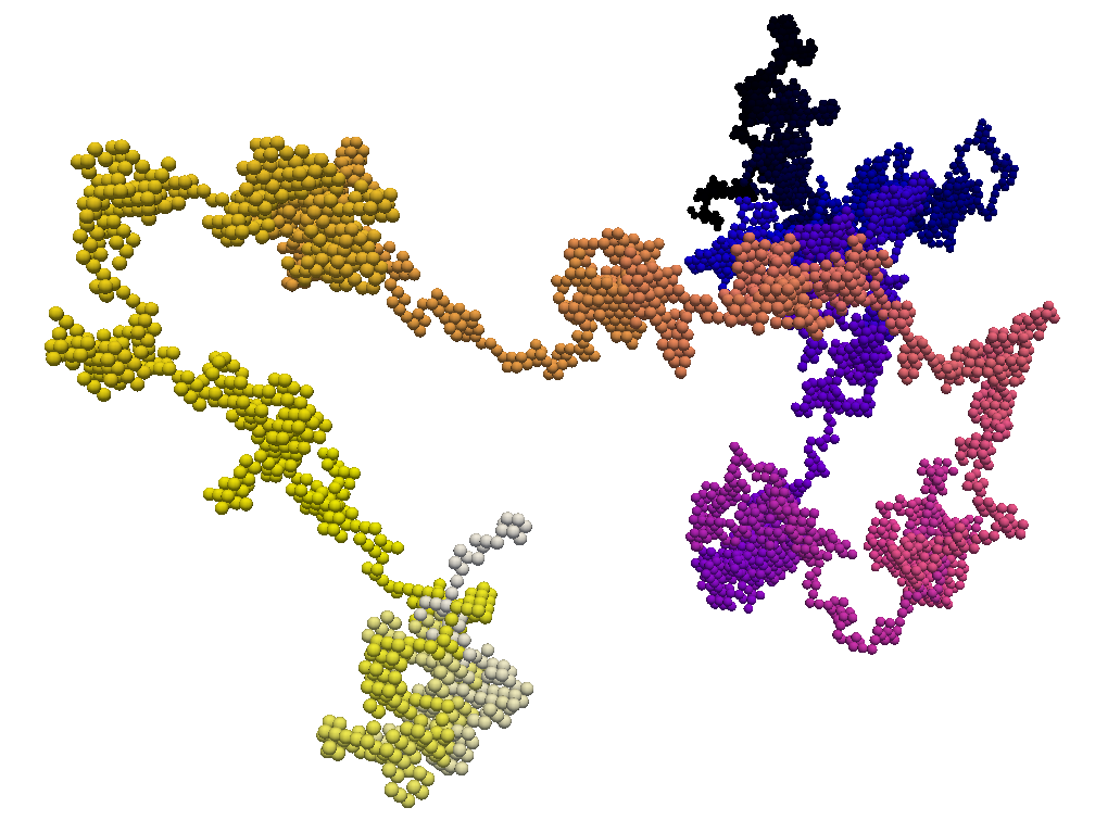
When using the ‘cmap:’ option to color the array, the hashblocks dictionary is built based on a linear relation between the chosen colormap and the values of the integers in the array, similar to how a gradient coloring would work. In the code block below, the RANDOMWALK.JSON model is drawn using the gnuplot2 colormap with an alpha of 1.
Note that this file generates a model that requires a substantial amount of memory, which may result in a longer rendering time.
model = vxm.Model()

model.load('randomwalk.json')
model.draw(coloring='cmap: gnuplot2, alpha:1',geometry='particles',background_color='w')
Colormap Block Coloring with Integer Tagging
The hashblocks map can be used in combination with the ‘cmap’ coloring option to selectively color-tag specific voxels based on their type. To accomplish this, we can modify the previous code block by adding a model.hashblocks declaration after model.load(). This will allow us to color the voxels represented by the integers 743, 500, and 256 in magenta, and the voxel represented by integer 2 in cyan.
model = vxm.Model()

model.load('randomwalk.json')

# add the hashblocks voxel assignments
model.hashblocks = {
  743: ['magenta',1],
  500: ['magenta',1],
  256: ['magenta',1],
  2: ['cyan',1]
}

model.draw(coloring='cmap: gnuplot2, alpha:1',geometry='particles',background_color='w')
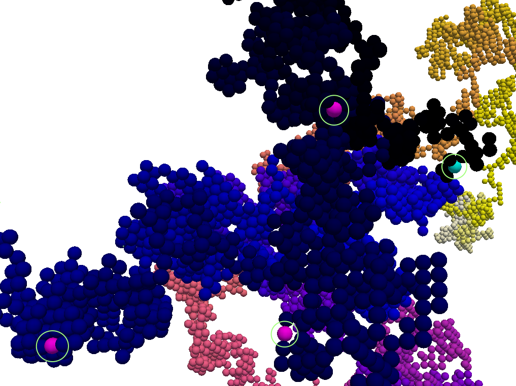
The ability to use the hashblocks map with the ‘cmap’ coloring option can be a valuable feature when we need to represent multiple relationships simultaneously. For example, we can use a gradient of values described by the colormap to color the array, while simultaneously highlighting specific voxels with hashblocks. This technique can have numerous applications in fields such as 3-D modeling, medical imaging, and coarse-grained molecular modeling, among others.
3-D Mapping of an Image
Here we map the synthetic topography LAND IMAGE (.png) to a
3-D model using the ImageMap method from the voxelmap.Model class.
#import packages
import cv2
import matplotlib.pyplot as plt

plt.imshow(cv2.imread('docs/img/land.png'))      # display fake land topography .png file as plot
plt.axis('off')
plt.show()

#import packages
import numpy as np
from matplotlib import cm

model = vxm.Model(file='docs/img/land.png')             # incorporate fake land topography .png file to voxelmap.Image class
print(model.array.shape)
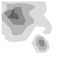
The image is then resized for the voxel draw with the matplotlib method i.e. Model().draw_mpl. This is done with cv2.resize, resizing the image from 1060x1060 to 50x50.
After resizing, we convolve the image to obtain a less sharp color shift between the different gray regions with the cv2.blur method:
model.array = cv2.resize(model.array, (50,50), interpolation = cv2.INTER_AREA)
print(model.array.shape)

model.array = cv2.blur(model.array,(10,10))    # blur the image for realiztic topography levels
plt.imshow(model.array)      # display fake land topography .png file as plot
plt.axis('off')
plt.show()
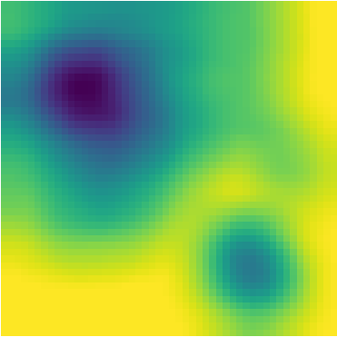
After this treatment, the resized and blurred image is mapped to a 3-D voxel model using the ImageMap method from the Model class:
model.array = model.ImageMap(12)              # mapped to 3d with a depth of 12 voxels
print(model.array.shape)

model.draw('none',background_color='#ffffff')
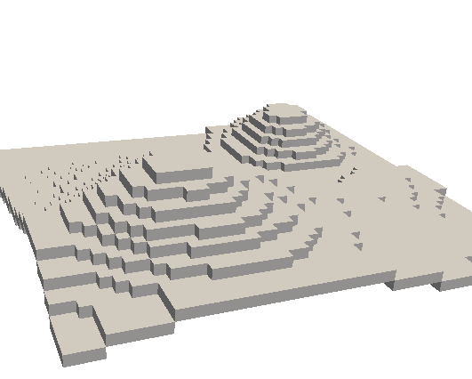
Low-Poly 3-D Mesh Mapping from Image
The ImageMesh method creates a low-poly mesh model from an Image using an algorithm developed by Andrew Garcia where 3-D convex hull is performed on separate “cuts” or sectors from the image (see: ImageMesh : A Convex Hull based 3D Reconstruction Method).
This can decrease the size of the 3-D model and the runtime to generate it significantly, making the runtime proportional to the number of sectors rather than the number of pixels. Sectors are quantified with the L_sectors kwarg, which is the length scale for the number of sectors in the grid.
We can see that the mesh model can be calculated and drawn with matplotlib plot=mpl option even from a large image of 1060x1060 without resizing:
import voxelmap as vxm
import cv2

model = vxm.Model(file='docs/img/land.png')   # incorporate fake land topography .png file

print(model.array.shape)

model.ImageMesh(out_file='scene.obj', L_sectors = 15, trace_min=5, rel_depth = 20, figsize=(15,12), plot='mpl')
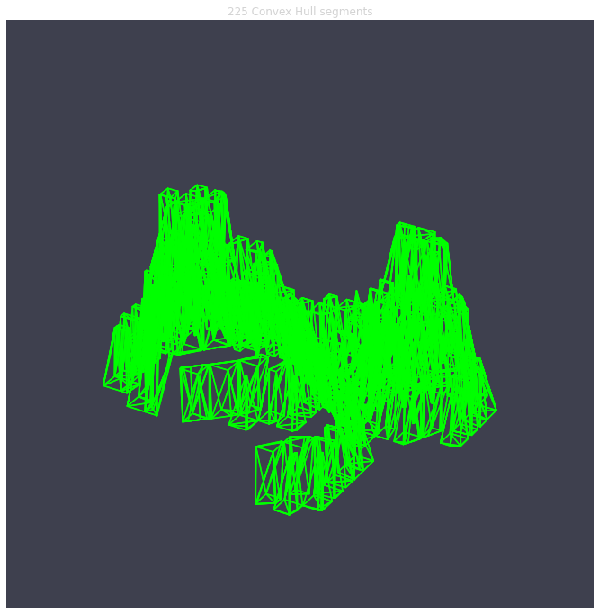
This ImageMesh transformation is also tested with a blurred version of the image with cv2.blur. A more smooth low-poly 3-D mesh is generated with this additional treatment. The topography seems more realistic:
model.array = cv2.blur(model.array,(60,60))    # blur the image for realiztic topography levels
model.ImageMesh(out_file='scene.obj', L_sectors = 15, trace_min=5, rel_depth = 20, figsize=(15,12), plot='mpl')
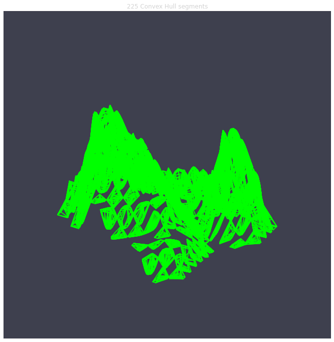
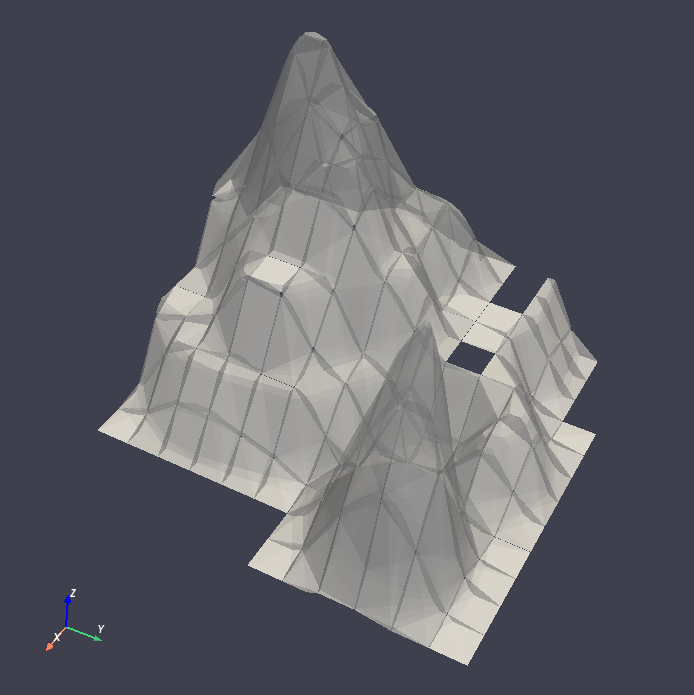
For a more customizable OpenGL rendering, img.MeshView() may be used on the above image:
import voxelmap as vxm
import numpy as np
import cv2 as cv

model = vxm.Model(file='docs/img/land.png')           # incorporate fake land topography .png file
model.array = cv.blur(model.array,(100,100))    # blur the image for realistic topography levels

# model.make()                                  # resized to 1.0x original size i.e. not resized (default)

model.ImageMesh('land.obj',  12, 14, 1, False, figsize=(10,10))

model.MeshView( alpha=0.7,background_color='#3e404e',color='white',viewport=(700, 700))
MarchingMesh : Turning Voxel Models to 3-D Mesh Representations
Click on the links below to save the files in the same directory you are running these examples:
The .txt files you downloaded were exported from Goxel projects.
Goxel is an open-source and cross-platform voxel editor which facilitates the graphical creation of voxel models. More information by clicking the icon link below.

We first load those .txt files with the below voxelmap methods:
import voxelmap as vxm
import numpy as np

'''process argisle.txt from Goxel'''
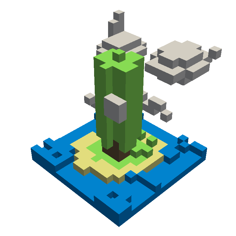
theIsland = vxm.Model()
theIsland.load('argisle.txt')
theIsland.array = np.transpose(theIsland.array,(2,1,0))    #rotate island
theIsland.draw('custom',background_color='white')

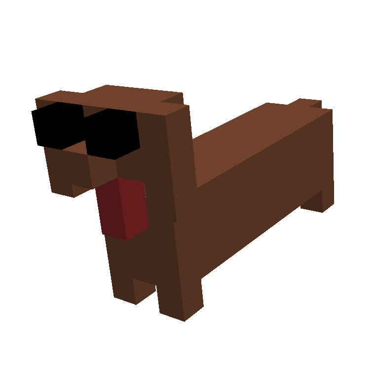
'''process dog.txt from Goxel'''
Dog = vxm.Model()
Dog.load('dog.txt')
Dog.array = np.transpose(Dog.array,(2,1,0))     #rotate dog
Dog.draw('custom',background_color='white')
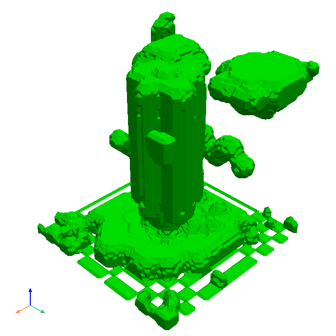
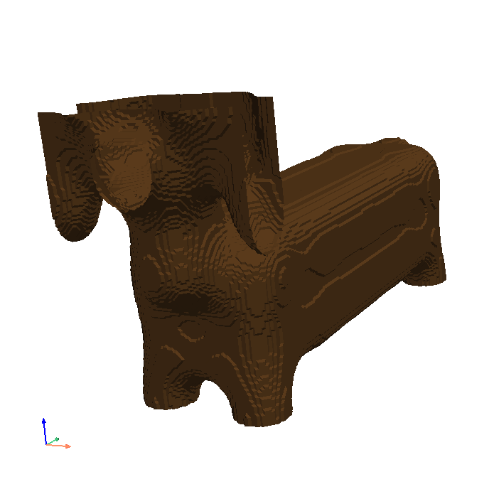
The voxel models can be transformed to 3D mesh representations with voxelmap’s Model().MarchingMesh method, which uses Marching Cubes from the scikit-image Python library.
'''MarchingMesh on island model'''
theIsland.array = vxm.resize_array(theIsland.array,(5,5,5)) #make array larger before mesh transformation
theIsland.MarchingMesh()
theIsland.MeshView(color='lime',wireframe=False,background_color='white',alpha=1,viewport=[700,700])

'''MarchingMesh on dog model'''
Dog.array = vxm.resize_array(Dog.array,(20,20,20)) #make array larger before mesh transformation
Dog.MarchingMesh()
Dog.MeshView(color='brown',wireframe=False,background_color='white',alpha=1,viewport=[700,700])
Notice the self.array arrays were resized in both objects with the global voxelmap.resize_array method. This was done to avoid the formation of voids that you still see on the dog mesh above.
The MarchingMesh method has a current limitation on small voxel models with low detail. It is not perfect, but this is an open-source package and it can always be developed further by
the maintainer and/or other collaborators.
Wavefront (.obj) file to 3-D Sparse Array
Voxelmap provides various features for converting Wavefront .obj files to its 3-D sparse arrays. However, the most straightforward approach is to use the global voxelmap.objcast method.
Cube Model
To begin, let’s download the simple_cube.obj model file. If you take a look at the file, you’ll see that it specifies the z, y, and x coordinates of each vertex. However, in order to convert this model to a voxel-based representation, we need to define the spacing between points, since we’re transforming from continuous coordinates to the discrete dimensions of a tensor.
To determine how the spacing affects the transformation from .obj to sparse array, we’ve provided a function below:
def draw_cube(spacing):

   array = vxm.objcast('simple_cube.obj',spacing) # Cast obj file as a point-cloud 3-D numpy array
   model = vxm.Model(array)
   model.draw(coloring='custom: black',wireframe=True,wireframe_color='w',background_color='#000000',voxel_spacing=(1,1,1))
>>> draw_cube(spacing=1)
(see below)

>>> draw_cube(spacing=0.5)
(see below)
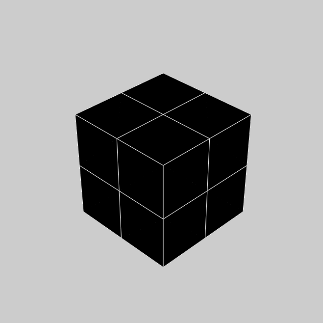
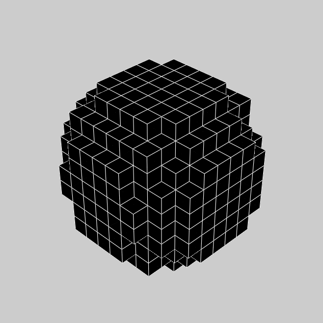
We can see a fractional spacing shows a more accurate model of a 2x2x2 supercube.
Sphere Model
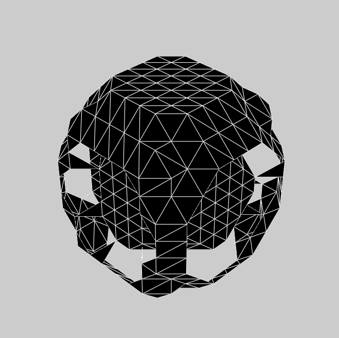
This second example demonstrates how voxelmap can be utilized to convert the sphere.obj MODEL into a discrete voxel array, which can then be triangulated using the MarchingMesh local method.
def sphere_ptcloud(spacing):

   # Draw as point cloud of voxels
   array = vxm.objcast('sphere.obj',spacing) # Cast obj file as a point-cloud 3-D numpy array
   model = vxm.Model(array)
   model.draw(coloring='custom: black',wireframe=True,wireframe_color='w',background_color='#000000',voxel_spacing=(1,1,1))

   # Draw as triangulated surface after applying Marching Cubes
   model.objfile= f"scene_marchingmesh{spacing}.obj"
   model.MarchingMesh()
   model.MeshView(wireframe=True,background_color='k',alpha=1)
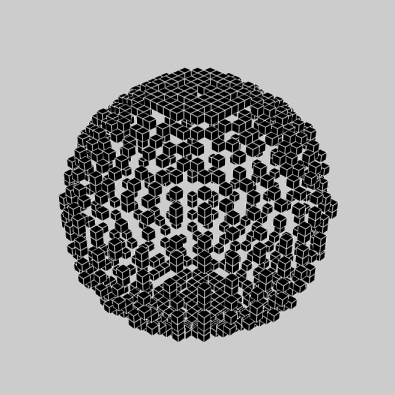
The spacing parameter is crucial when working with the sphere.obj model, which has fractional coordinates between 0 and 1. The transformation from continuous coordinates to a discrete tensor space involves floor-dividing the coordinates, so using a spacing of 1 is likely to result in an unhelpful sparse 3-D tensor for voxel point cloud modeling. To address this issue, we initially set the spacing to 10 and obtained the following results.
>>> sphere_ptcloud(spacing=10)
(see below)
It is important to note that the spacing parameter plays a crucial role in transforming the .obj model to a discrete tensor space, especially when the model has fractional coordinates between 0 and 1. Setting a spacing value of 1 might not produce a useful sparse 3-D tensor for voxel point cloud modeling. In this example with the sphere model, we set the spacing to 10 and obtained satisfactory results.
>>> sphere_ptcloud(spacing=30)
(see below)
The MarchingMesh method typically output a Wavefront (.obj) file named scene.obj as default, but users can specify a different name by changing the
objfile variable in the constructor of the voxelmap.Model class. Once the file is generated, it can be edited in software like Blender by importing it.
The above commands generated 2 MarchingMesh .obj files, scene_marchingmesh10.obj and scene_marchingmesh30.obj for the different spacings chosen. These files can be imported simultaneously to a
Blender project, and they look like this:
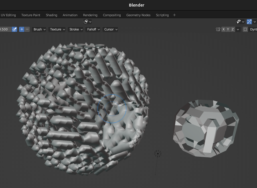
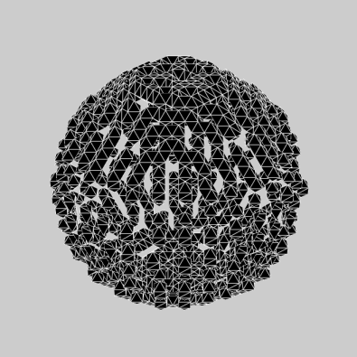
The larger spacing between voxels in a sphere can be observed to result in a larger overall size of the sphere.
3-D Model Numpy Manipulation and Blender Integration
What if we wanted to make a modification to the .obj file with Numpy and then save the new modified model as an .obj file for additional treatment in other software like Blender? Here we show a use case for that. Let’s take the above sphere_ptcloud() function and make the following changes:
def sphere_skewer():

   array = vxm.objcast('sphere.obj',30) # Cast obj file as a point-cloud 3-D numpy array

   #Numpy manipulation
   for i in range(30):
       x,y = np.random.randint(0,np.min(array.shape),2)
       array[x,y,:] = 1

   vxm.Model(array).save('pillars.obj')    #save the array as an .obj file

   model.objfile= f"pillars_mesh.obj"
   model.MarchingMesh()
   model.MeshView(wireframe=True,background_color='k',alpha=1)
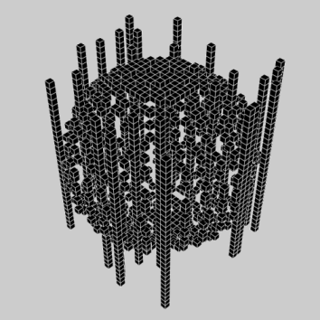
The above code block loads the sphere.obj file, and casts it as a point-cloud 3D numpy array using
the objcast method. It then makes 30 pillars in random x-y coordinates using Numpy. After this, the modified Numpy
array containing the voxel model can be saved back to an .obj format as a NEW FILE using the local save method
of the voxelmap.Model class.
The new pillars.obj file can be viewed with voxelmap with the below command
>>> vxm.MeshView('pillars.obj',alpha=1,wireframe=True)  # load for view with the global MeshView method
(see below)
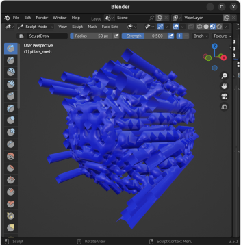
And with Blender importing pillars_mesh.obj with the Import tool. Below are the outputs from the voxelmap (left) and the
Blender (right) approach:
3-D Voxel Model Reprocessing
Here we do some reprocessing of the above voxel models. Note that here we use the draw_mpl method, which is voxelmap’s legacy method for voxel modeling and not its state-of-the-art. For faster
and higher quality graphics with more kwargs / drawing options, use voxelmap’s draw method instead.
Re-color with custom colors
using the hashblocks_add() method
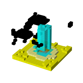
theIsland.hashblocks_add(1,'yellow',1)
theIsland.hashblocks_add(2,'#333333',0.2)
theIsland.hashblocks_add(3,'cyan',0.75)
theIsland.hashblocks_add(4,'#000000')

theIsland.draw_mpl('custom',figsize=(5,5))

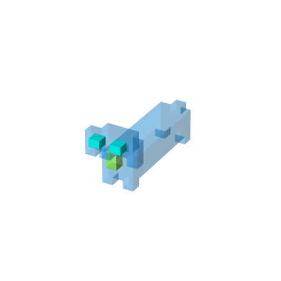
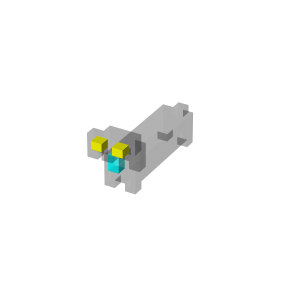
Dog.hashblocks = theIsland.hashblocks
print('black dog, yellow eyes, cyan tongue')
Dog.draw_mpl('custom',figsize=(5,5))
defining them directly in the hashblocks dictionary
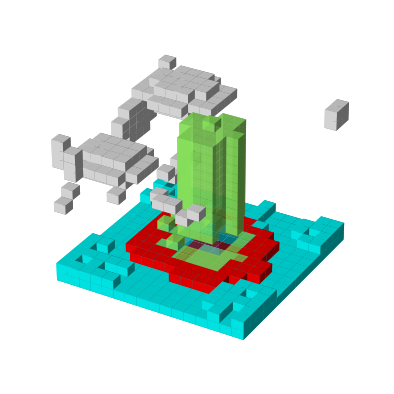
theIsland.hashblocks = {
      1: ['cyan', 1],
      2: ['#0197fd', 0.25],
      3: ['#98fc66', 0.78],
      4: ['#eeeeee', 1],
      5: ['red', 1]}

theIsland.draw_mpl('custom',figsize=(7,7))
Save and Load Methods for voxelmap Model objects
Save the ghost dog model
If you’d like to save an array with customized color assignments, you may do so now with the Model().save() method. This method saves the array data as a DOK hashmap and integrates this DOK hashmap with the Model.hashblocks color information in a higher-order JSON file format:
#re-define colors for a ghost dog
Dog.hashblocks = {
      1: ['cyan', 1],
      2: ['#0197fd', 0.25],
      3: ['#98fc66', 0.78],
      4: ['#eeeeee', 1]}

#save
Dog.save('ghostdog.json')
Load ghost dog model
The Model().load() method processes the array and color information to a blank Model object. To load this data into a “blank slate” and re-draw it, type the following:
# defines a blank model
blank = vxm.Model()
print(blank.array)
print(blank.hashblocks)

blank.load('ghostdog.json')

print(blank.array[0].shape)
print(blank.hashblocks)
blank.draw_mpl('custom',figsize=(7,7))
